
When it comes to Microsoft Excel, most people fall into one of two categories. There are those that love it and can’t live without it, and there are others who hate it and are completely intimidated by it. In today’s era of data, learning how to use Excel to be more productive is important. Despite the fact that there are a vast amount of other applications available for data storage and manipulation, Excel remains one of the best available for businesses, simply because of how much it can do.
Many people, however, do not use Microsoft Excel to its full extent.
Here we share 10 Excel tips and tricks that can help you become more productive when using Excel in the workplace.
Excel tips and tricks #1: Use Excel’s templates
Designing the structure of your information can be tedious and time-consuming. Fortunately, Excel offers a variety of ready-made templates for various tasks, so you don’t have to create a design from scratch.
To access Excel’s templates, go to File > New > From Template
Here you can find any number of templates, from monthly budgets, to financial statements to expense reports and budget plans allowing you to view metrics like revenue, operating profit, interest, depreciation, net profit, and quarterly trends at a glance. There are even templates for employee timesheets, a work schedule for your employees, and a travel planner. Plus, the templates can be customized to suit your requirements.
Excel tips and tricks #2: Use keyboard shortcuts
There are many keyboard shortcuts in Excel to cut down on the time it takes to achieve certain tasks. There are just a selection of the many available:
- Select only visible cells and not hidden cells: select the range you want and then hit Alt + ; to exclude those hidden entries. Mac equivalent: Cmd + Shift + Z
- Find the next matching entry: to open the Find and Replace window, use Ctrl + F. Use Shift + F4 to find the next matching entry once you have typed in the match you are looking for. To find the previous match, just use Ctrl + Shift + F4. These keyboard shortcuts will work whether the Find and Replace Window remains open or is closed. Mac equivalent: Next: Cmd + G | Previous: Cmd + Shift + G
- Enter a formula/value in all selected cells: copy data from one cell in a selection to the remainder of the selection by hitting Ctrl + Enter after selecting the cells you want affected and typing in your value or formula in the selected cell. This will copy your formula to all of the other selected cells. Mac equivalent: Ctrl + Enter
- Modify the cell style: to change the style of a cell, press Alt + ‘ (apostrophe) to bring up the Style Window. From there you can alter the formatting. Mac equivalent: Cmd + Shift + L
- Selecting cells with differences: you can identify the cells from a selected range that are different from the original selected cell using Ctrl + Shift + \ (backslash). This is for differences within a column. If you want to identify differences within a row, use Ctrl + \. Mac equivalent: Column: Ctrl + Shift + \ | Row: Ctrl + \
Excel tips and tricks #3: Use date and time in your pivot tables
The term ‘pivot tables’ can strike fear into the heart of even the most savvy business person! But they are nothing to be afraid of, and are, in fact, one of the most useful business tools you will come across within Excel. Pivot tables can help you create dynamic summary reports from raw data very easily, all in a drag-and-drop interface.
This post is focused on Excel tips and tricks however, so we will assume that you are already using pivot tables and don’t need a tutorial!
Using date and time as a metric within pivot tables is one of the most powerful ways to analyze the data. In most cases, business analysis will be on a monthly, quarterly, or annual basis. If your data is listed by day, you need to convert the dates.
This is easily done. In your pivot table, select one of the cells that contains a date in the day format, right click and choose Group. You can now select how you want to group your dates for more meaningful analysis and insights.
Excel tips and tricks #4: Insert live data from the Internet into your worksheets
In Excel 2010 and later you can automatically update your worksheets with time sensitive data directly from the Internet. For example, you may need to include the current daily exchange rate, which can be pulled in automatically rather than having to be updated manually everyday. Other information that can be added automatically could include stock prices, flight information, weather—essentially anything that updates on a regular basis.
- If you’re using 2010, download and install the Power Query Add-In. This is already built into 2013 and later.
- Click Power Query (or Data > New Query > From Other Sources > From Web)
- In the From Web box, enter the website URL. Click OK.
- Power Query will scan the webpage, and load the data in the Navigator Pane under the Table View.
- Select the table you want to connect to by clicking it from the list.
- Click Load, and the web data will be seen on your worksheet.
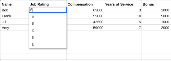
Excel tips and tricks #5: Use list data
If some cells should only be populated with one of a specific list of values, it’s easy to create a list for the user to choose from.
Select the cells that the list choices will be applied to.
Go to Data > Data Validation.
Under Allow, choose List and then type the available options under source, separated with a comma. Alternatively, if you have your list in the spreadsheet, select the range and click OK. Now, when filling the data, users can choose from the drop down list, which is often faster than having to type out full answers.
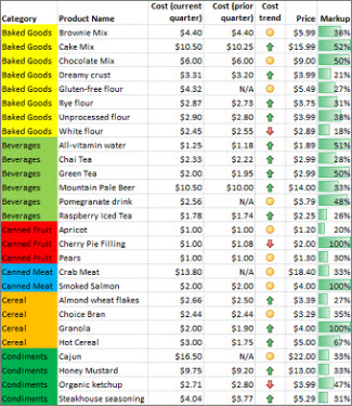
Excel tips and tricks #6: Highlight cells with conditional formatting
Conditional formatting allows you to highlight interesting cells or ranges of cells so that it’s easier to analyze the data. You can see trends at a glance, detect unusual values and better visualize data by using data bars, color scales, and icon sets that correspond to specific variations in the data. With conditional formatting, a condition, or a set of conditions are set that will change the cell’s appearance once met.
Excel has many built-in conditions, and you can also create your own. Here are three of the most popular:
- Color scales are visual guides that help you understand data distribution and variation. The shade of the color represents higher or lower values.
- Icon sets can be used to annotate and classify data into categories separated by a threshold value. For example, in the 3 Arrows icon set, the green up arrow represents higher values, the yellow sideways arrow represents middle values, and the red down arrow represents lower values.
- Data bars are useful in spotting higher and lower numbers, especially with large amounts of data. The longer the bar, the higher the value it represents.
To enable Conditional Formatting, select the cells that you would like to be impacted by the formatting.On the Home tab, in the Styles group, click the arrow next to Conditional Formatting, and then click Color Scales, Data Bars, or Icons.
Excel tips and tricks #7: View a cell’s dependencies
Complex worksheets can include formulas and values that impact several other cells. Before you know it, you’ve made a small change to one cell and you’re faced with multiple errors in other cells. It’s helpful to understand the relationship between cells—especially if it’s a spreadsheet you didn’t personally create.
Select a cell in your worksheet and then press Ctrl-Shift-] and all of the cells that are dependent on the selected cell will be highlighted.
Bonus tip: With a cell selected, click on Trace Dependencies from the Formula ribbon and you’ll see lines from the cell to the dependent cells. Click Trace Dependencies a second time and you’ll see the dependencies of those cells.
Excel tips and tricks #8: Plot data with geographical locations on a map
The Map Charts feature in Excel reads columns with geographic locations in your spreadsheet and automatically turns them into stunning, dynamic color-coded maps. Learn more about Map Charts here.
Excel tips and tricks #9: Get familiar with some useful functions
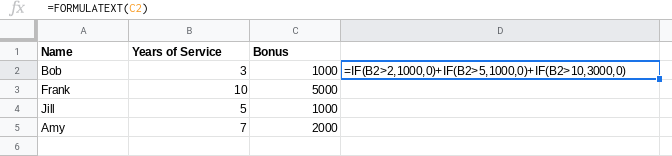
The FORMULATEXT and the N function
This tip is actually going to make the people using the spreadsheet after you more productive. There’s nothing worse than inheriting a complex spreadsheet and having no idea how it was set up. It’s very quick and easy to document your worksheet using FORMULATEXT and the N function, but it’s not something that everyone knows how to do, or why for that matter.
In the cell next to your formula, use the function =FORMULATEXT(cell number). E.g. =FORMULATEXT(C9). This will display your formula, making it easy to know at a glance how that value was calculated. Here is a very simple example:
=(YOUR FORMULA GOES HERE)+N(“YOUR FORMULA DESCRIPTION GOES HERE”).
The resulting value of the formula won’t change, but you have now described the formula for future reference! Here you can see the N function is used to let other users know that this special bonus is calculated based on years of service.
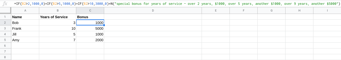
So, while documenting the formulas in your spreadsheet probably isn’t very high on your list of things to do, taking a few moments to do so will make other people’s lives much easier if they take over your spreadsheet, and it will even help you if you even need to remember how or why the spreadsheet was set up years down the road.
The VLOOKUP Function
VLookup is a powerful Excel function used when you need to quickly find specific data within a large table, for example, names, phone number, specific value etc. For example, you could look for the first name and last name of a client based on the account number you have.
Note: VLOOKUP is designed to retrieve data in a table organized into vertical rows, where each row represents a new record. If you have data organized horizontally, use the HLOOKUP function.
Lookup values must appear in the first column of the table, with lookup columns to the right.
The VLookup formula is
=VLOOKUP (value, table, col_index, [range_lookup])
- value – The value to look for in the first column of a table.
- table – The table from which to retrieve a value.
- col_index – The column in the table from which to retrieve a value.
- range_lookup – This is an optional argument that allows you to search for the exact match of your lookup value without sorting the table.TRUE = approximate match (default). FALSE = exact match.
The CONCATENATE Function
The CONCATENATE function allows you to combine text from different cells into one cell. For example, you could combine first names and last names from separate columns into one column. To combine the text in cells A2 and B2, your formula would be:
=CONCATENATE(A2, B2)
If you need to add a space between the two combined values, simply add another argument: ” ” (two double quotes around a space). Make sure the three arguments are separated by commas:
=CONCATENATE(B2,” “,A2)
The IFERROR function
The IFERROR function returns a custom result when a formula generates an error, and a standard result when no error is detected.
The formula would be:
=IFERROR (value, value_if_error), where:
- value – The value, reference, or formula to check for an error.
- value_if_error – The value to return if an error is found.
For example, if A1 contains 10, B1 is blank, and C1 contains the formula =A1/B1, the following formula will catch the #DIV/0! error that results from dividing A1 by B1:
=IFERROR (A1/B1,”Please enter a value in B1″)
Excel tips and tricks #10: Make use of The Flash Fill option
Flash Fill (available in Excel 2013 and later) automatically fills your data when it senses a pattern. For example, you can use Flash Fill to separate first and last names from a single column, or combine first and last names from two different columns (instead of using the Concatenate function mentioned above). This can save a lot of tedious manual work.
To turn Flash Fill on, go to Tools > Options > Advanced > Editing Options > check the Automatically Flash Fill box.
Most people are trying to be more productive and efficient throughout their day, and Microsoft Excel can help achieve this goal, however there are hundreds of functions and features that will largely go unused by most people. The 10 Excel tips and tricks presented above can increase your data handling speed and accuracy, saving you time and money.